Sizing¶

Appropriate sizing of a simulation environment is more art than science but we can use several tools in the RKnot package and the scientific literature to approximate appropriate attributes and initial conditions.

Our main guides for appropriate sizing:

Actual $R_0$ should be close to target $R_0$
Contact rate should follow a gamma distribution with parameters found in the Hutch model.
$R_0$ distribution should replicate the Endo distribution.

Our main tools for adjusting contact rates and $R_0$ distribution are:

Importance of Distributions¶

Both the distribution of contacts and individual $R_0$ are important considerations when formulating a realistic model of viral spread.

In terms of contacts, both frequency and timing are important. All else equal, an infected individual will cause more secondary infections if they have more contacts. BUT an infected individual contacting the same number of people at two different times is likely to cause more secondary infections at the time of greater viral load.

The SIR model makes many simplifying assumptions that fail to replicate real world spread. In particular, SIR is characterized by:

Uniform, average contact rates
Constant transmission risk

These two assumptions result in normally distributed contact rates among all individuals in an environment and normally distributed individual $R_0$.

Endo et al, however, have suggested that 70%+ of all sars-cov-2 infections lead to :math:`underline{text{NO}}` secondary infections. And that the vast majority of secondary infections are due to a small minority of super-spreader carriers.

To account for this, the Hutch team modelled contacts with a gamma distribution, which (relative to the Gaussian) favors many more instances of 0 contacts, but also allows for a very long tail of large contacts depending on the dispersion parameter.

Constant Contact Rate and Transmission Risk¶

To replicate the Hutch approach in RKnot, we must first understand contact and transmission dynamics in more generalized scensarios.

We will use the looper helper function to run 1,000 interations of simulations for two environments:

Equal Mover scenario with density=1.
Equal Mover with density=5

from rknot.notebook import looper

params = dict(density=1, R0=2.5, infdur=14, days=14, sterile=True,)
group = dict(name='all', n=10000, n_inf=1, ifr=0, mover='equal',)
contacts_1, nsecs_1, _, __ = looper(n=1000, groups=group, **params)

params['density'] = 5
contacts_5, nsecs_5, _, __ = looper(n=1000, groups=group, **params)

Daily Contact Distribution¶

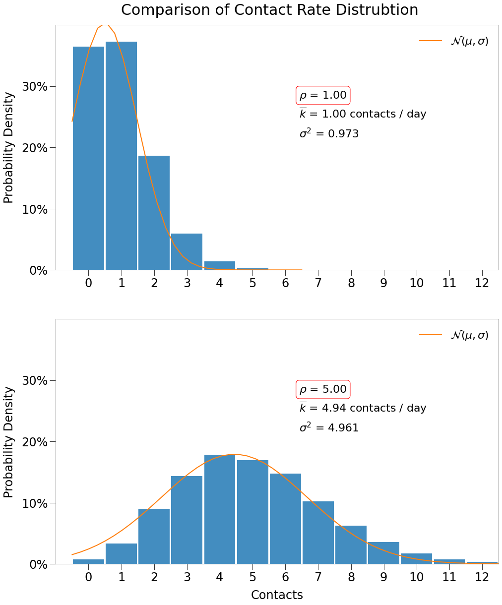
The daily contact mean and variance are found simply as contacts_1.mean(), contacts_1.var(), etc. For each environment, the mean, variance, and density are about equal.

Seen as per table below:

Density, $\rho$	$\overline{{k}}$	$\sigma^2$
1	0.9973	0.9731
5	4.9436	4.9607

We can also see below that daily contacts are normally distributed in both environments (technically, binomially distributed as discussed here).

SIR auto-adjusts for density

When $R_0$ and infdur are provided, RKnot will automatically scale the transmission risk such that the environment will produce the desired R0, regardless of the density. We can see this in the next comparison.

Curve Details¶

In the table below, we show the results of the simulations across the two environments.

	$\rho$ = 1	$\rho$ = 5
Peak	40.1%	38.6%
HIT	61.6%	59.5%
Total	82.4%	79.5%
Days to Peak	66	64

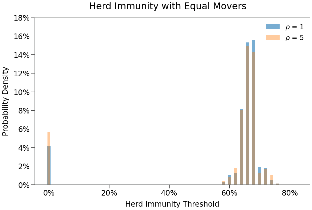
Both environments do a decent job of meeting the expected HIT. With $R_0$ of 2.5 (and assuming SIR conditions), HIT is generally understood to be $1 - 1/R_0 = 1 - 1 / 2.5 =$ 60%

That said, this is in part due to the fact that ~10% of all simulations ended with no secondary infections, so most simulations ended with between 65% and 75% HIT as per below:

Secondary Infection Distribution¶

Now, we compare the $R_0$ generated in each simulation of the two environments. Each chart below shows the actual number of secondary infections generated in each of 1,000 simulations with two different distributions overlayed.

a Binomial distribution deterimined as follows:

\[\begin{split}\begin{equation} B(n,p) = B(\text{infdur} * \overline{k}, \frac{R_0 / \text{infdur}}{\overline{k}}) \\where: n = \overline{c} = \text{infdur} * \overline{k} \\ p = R_0 / \overline{k} / \text{infdur} \\ \overline{c} = \text{average total contacts} \\ \overline{k} = \text{average daily contact rate} \end{equation}\end{split}\]

$\frac{R_0}{\textit{infdur}}$ number of infections occuring during each day and $\frac{R_0 / \textit{infdur}}{\overline{k}}$ infections occuring per contact.

the Endo distribution determined as follows:

\[\begin{split}\begin{equation} \textit{Endo}(R_0, \omega) \\\textit{where: }\omega \textit{ is the overdispersion parameter} \end{equation}\end{split}\]

The Endo model is fairly complex so readers are encouraged to research it here. The paper determined an optimized value of $\omega$ of 0.1 sars-cov-2, which will be used for our purposes.

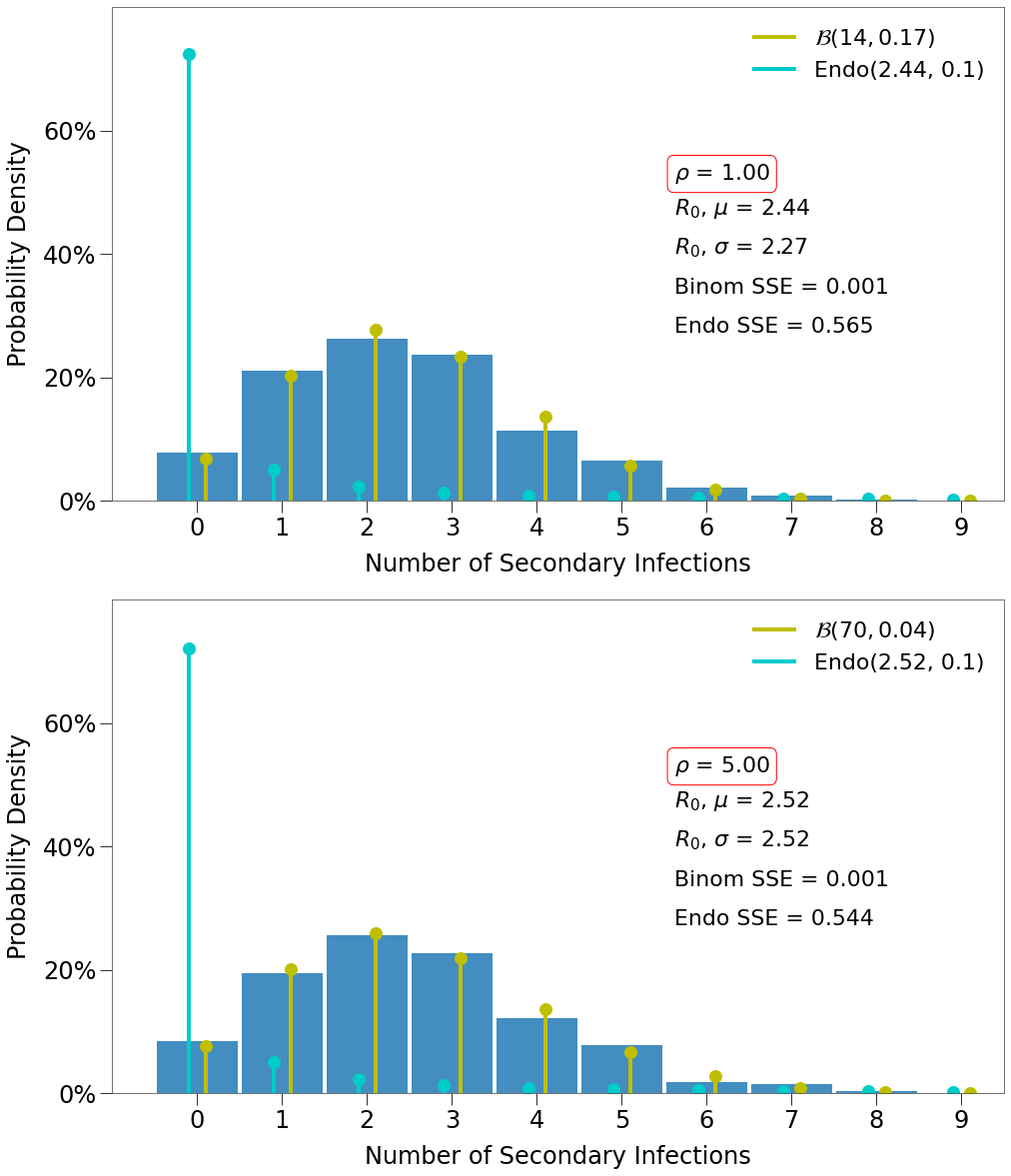
We can see both environments do a good job of generating ~2.5 secondary infections, on average.

We also see that both have $R_0$ distributions that fit the binomial distribution, not the Endo.

Movement Changes¶

We have seen the impact of density on the properties of the spread. Now we investigate the impact of movement patterns.

Local Bias¶

local patterns restrict the movement of a dot to only the nearest available locations. This is achieved using a geometric distribution with the p parameter governing the amount of restriction. The larger the p, the greater the restriction.

This is illustrated below:

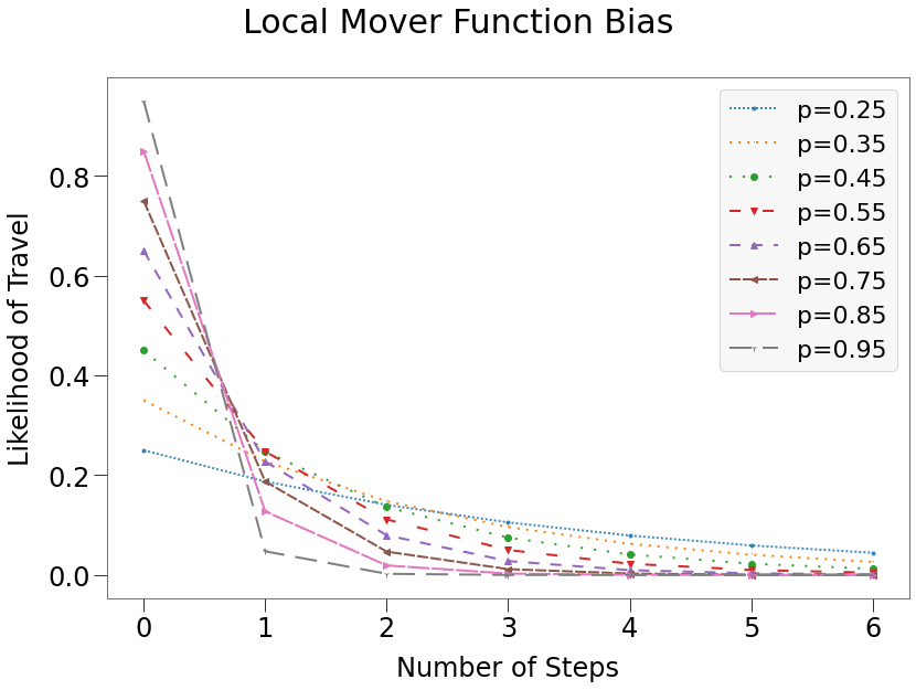
There are several pre-defined mover functions, which can be utilized by providing a string or integer value to the mover attribute of a Group. The local mover function, for instance, utilizes a geometric distribution with p-value of 0.6.

The mover attribute also accepts a float value, which is then provided as the specified p-value to a geometric distribution.

With this feature, we can generate simulations across a range of p-values.

Then, we can use the helper function find_all_contacts to generate a 2d array of the number of the contacts on each tick for every dot in each sim. Then multiply the contacts the transmission risk curve to get the expected $R_0$ for every dot in the sim as though they were infected initially.

Repeat this for each p-value. Here, we cannot use looper, because the properties of each sim will change slightly, but we can use the recycler decorator to simplify the loop and pass existing server and worker actors if they are available.

from rknot import Sim
from rknot.sim import recycler
from rknot.notebook import find_all_contacts

params = dict(density=.75, R0=2.5, infdur=14, days=14, sterile=True, n_workers=1)
group = dict(name='all', n=10000, n_inf=1, ifr=0,)

p = np.concatenate((p, np.linspace(0.96, .99, 4)))

dotlogs = np.zeros(shape=(p.shape[0], params['days']+1, group['n'], len(ML)), dtype=np.int32)
all_contacts = np.zeros(shape=(p.shape[0], group['n'], params['days']), dtype=np.int32)
tmrs = np.zeros(shape=(p.shape[0], params['infdur']))

sim_cycler = recycler(p.shape[0])
for i in trange(p.shape[0]):
    group['mover'] = p[i]
    sim = sim_cycler(groups=group, pbar=False,  **params)
    sim.run(dotlog=True, pbar=False)
    dotlogs[i] = sim.dotlog
    all_contacts[i] = nbf.find_all_contacts(sim.dotlog, MLNB)
    tmrs[i] = sim.tmrs

contact_means = all_contacts.sum(axis=2).mean(axis=1) / params['days']
eR0s = np.zeros(all_contacts.shape[0])
for i in range(eR0s.shape[0]):
    eR0_by_dot = tmrs[i] * all_contacts[i]
    eR0_mu = eR0_by_dot.sum(axis=1).mean()
    eR0s[i] = eR0_mu

We can then chart $E(R_0)$ against p-value to see the impact of restricting movement on spread.

Further, we show the change in mean contacts against p-value (which is a similar curve) and fit that curve to a 5-degree polynomial. This will be helpful in building Complex Environments.

We can also easily accomodate densities less than one by simply multiplying the polyfit parameters by the density.

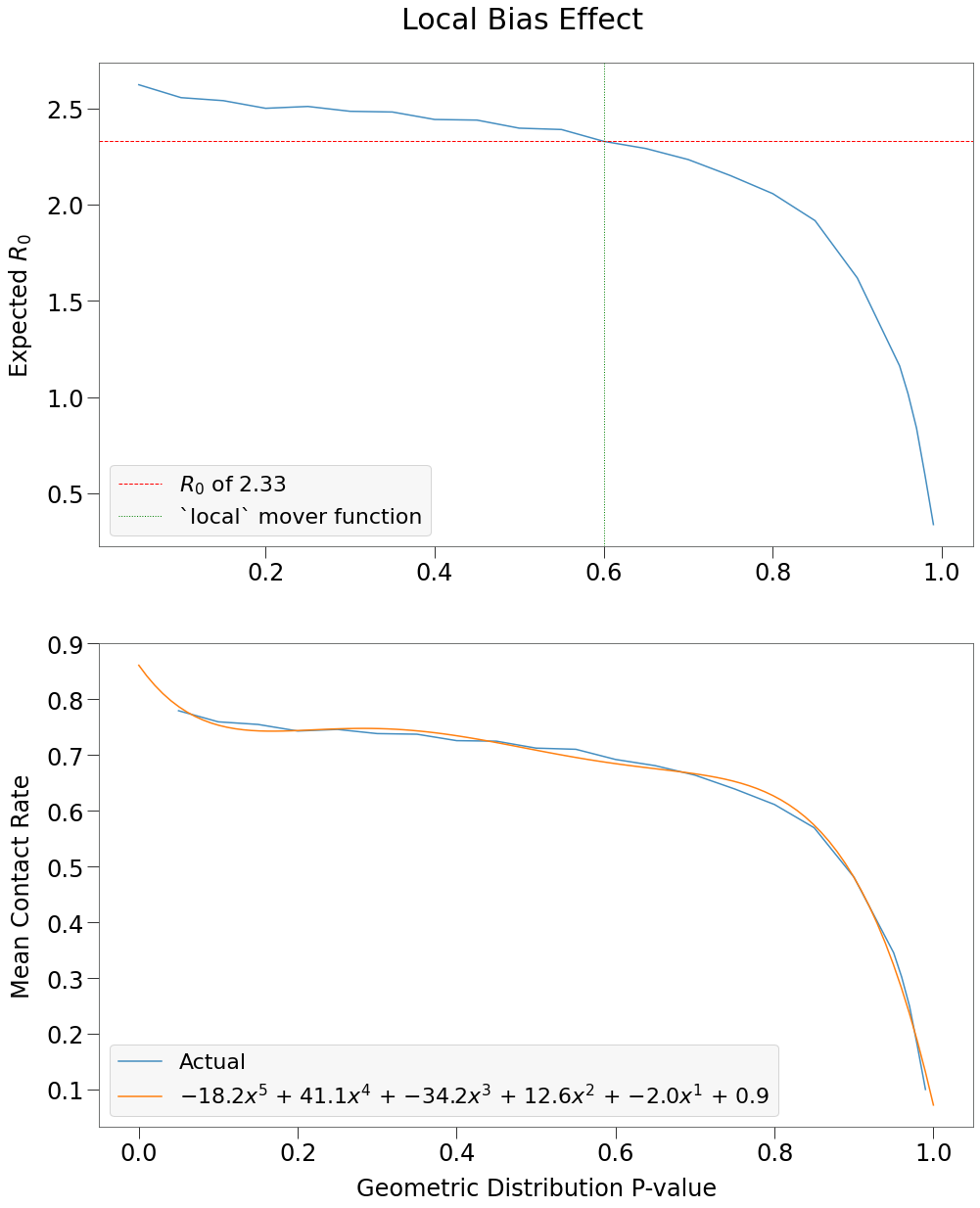
We see that $R_0$ has an inverse relationship to restricted movement (i.e. spread increases as populations become more well-mixed). This, of course, makes sense and is a fundamental premise of viral spread theory.

$\underline{\text{However}}$ what cannot be overlooked is how closely $R_0$ in a moderately restricted environment resembles a completely well-mixed environment. And yet we know that the local mover function (with p-value of 0.6) results in a very different long-term spread curve.

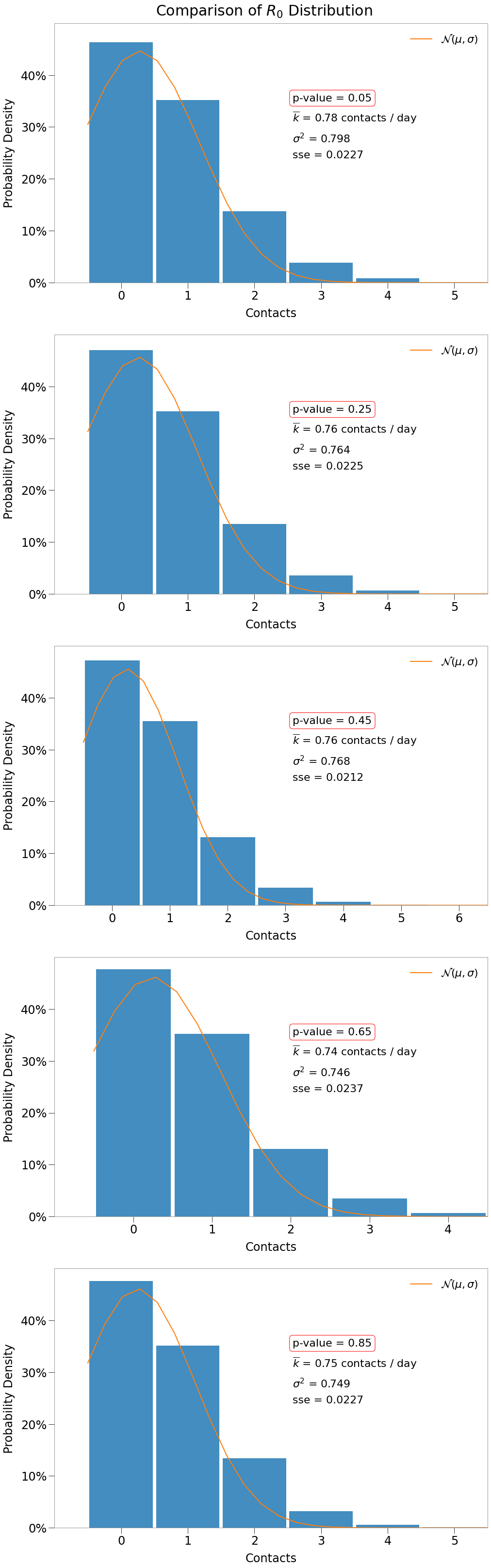
Further, each p-value results in normally-distributed contacts. We show this for a handful of p-values below.

Interplay of Movement and Density¶

We can also run each p-value against a range of densities.

params = dict(
    R0=2.5,
    infdur=14,
    days=14,
    sterile=True,
    pbar=False,
    pbar_leave=False,
    reset_env=True,
)
group = dict(
    name='all',
    n=10000,
    n_inf=1,
    ifr=0,
)
densities = np.array([.5, .75, 1, 2.5, 5])

dotlogs = np.zeros(shape=(
        p.shape[0], densities.shape[0], params['days']+1, group['n'], len(ML)
    ), dtype=np.int32
)
all_contacts = np.zeros(shape=(
        p.shape[0], densities.shape[0], group['n'], params['days']
    ), dtype=np.int32
)
tmrs = np.zeros(shape=(densities.shape[0], params['infdur']))

n_iters = p.shape[0]*densities.shape[0]
pbar = tqdm(total=n_iters)
sim_cycler = recycler(n_iters)
for i in range(p.shape[0]):
    group['mover'] = p[i]
    for j in range(densities.shape[0]):
        sim = sim_cycler(groups=group, density=densities[j], **params)
        sim.run(dotlog=True, pbar=False)

        dotlogs[i, j] = sim.dotlog
        all_contacts[i, j] = find_all_contacts(sim.dotlog, MLNB)
        tmrs[j] = sim.tmrs

        pbar.update(1)

Then find the expected $R_0$ for each combination:

eR0s = np.zeros(shape=(all_contacts.shape[0], all_contacts.shape[1]))
for i in range(eR0s.shape[0]):
    for j in range(eR0s.shape[1]):
        eR0_by_dot = tmrs[j] * all_contacts[i, j]
        eR0_mu = eR0_by_dot.sum(axis=1).mean()
        eR0s[i, j] = eR0_mu

And below we show $R_0$, contact $\mu$, and contact variance for a subset of the p-value/density combinations.

		$\rho$ = 0.5			$\rho$ = 0.75			$\rho$ = 1.0			$\rho$ = 2.5			$\rho$ = 5.0
p-value	$R_0$	$\overline{k}$	$\sigma^2$	$R_0$	$\overline{k}$	$\sigma^2$	$R_0$	$\overline{k}$	$\sigma^2$	$R_0$	$\overline{k}$	$\sigma^2$	$R_0$	$\overline{k}$	$\sigma^2$
0.05	2.60	0.52	0.52	2.61	0.78	0.80	2.60	1.04	1.08	2.54	2.48	2.55	2.52	4.98	5.12
0.20	2.51	0.50	0.50	2.52	0.75	0.75	2.51	1.00	1.00	2.55	2.50	2.60	2.57	5.09	5.56
0.35	2.45	0.49	0.49	2.48	0.74	0.73	2.48	0.99	1.01	2.52	2.46	2.46	2.53	5.00	5.20
0.50	2.41	0.48	0.48	2.41	0.72	0.70	2.43	0.97	0.96	2.50	2.44	2.41	2.51	4.96	4.99
0.65	2.30	0.46	0.45	2.32	0.69	0.67	2.29	0.92	0.88	2.50	2.44	2.46	2.51	4.96	5.06
0.80	2.04	0.41	0.40	2.05	0.61	0.58	2.03	0.81	0.75	2.54	2.48	2.58	2.50	4.94	4.95
0.95	1.17	0.23	0.22	1.14	0.34	0.33	1.17	0.47	0.43	2.50	2.44	2.45	2.48	4.90	4.66
0.98	0.64	0.13	0.12	0.60	0.18	0.17	0.61	0.25	0.23	2.49	2.43	2.40	2.47	4.89	4.74

The table above has some interesting properties:

As expected, mean contacts, $\overline{k}$, increases with density.
Also, for densities of 1 or less, $\overline{k}$ decreases with p-value.
Also, for densities of 1 or less, $R_0$ decreases with density.

HOWEVER, when density > 1, all of the values remain almost constant for each density regardless of p-value. When a grid is overloaded with dots, by definition the same number of dots are expected at each location regardless of the movement pattern (on average).

Location Clustering¶

We should also mention the phenomena of dot clustering. We can determine how many different locations are occupied by at least one dot at each tick as follows:

[27]:

unq_locs = np.zeros(shape=dotlogs.shape[:3])
for i in range(dotlogs.shape[0]):
    for j in range(dotlogs.shape[1]):
        for k in range(dotlogs.shape[2]):
            unq_locs[i,j,k] = np.unique(dotlogs[i,j,k,:,ML['loc_id']]).shape[0]

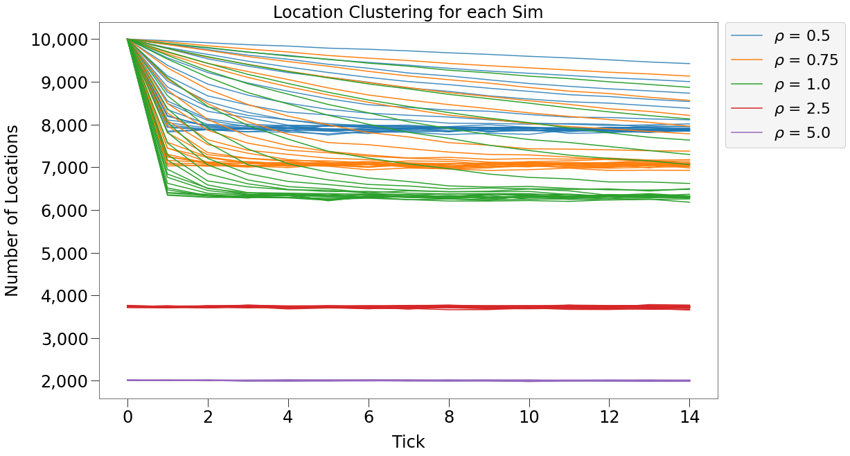
In the chart below, we can see that each sim with density < 1, starts with dots occupying 10,000 unique locations (so each dot gets its own location), but over time dots cluster to a smaller number of locations.

The clustering appears asymptotic to a long-term value. That value appears to be inversely related to the density (so lower density means more locations and less clustering). And the speed at which that value is reached is related to the p-value.

For sims with density > 1, there is no clustering.

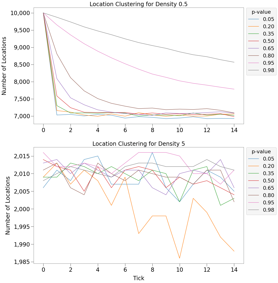
Below we more clearly see the relationship between p-value and speed of clustering:

For density of 0.5:
- p-value is inversely related to clustering speed. i.e. movement patterns with higher p-values cluster slower
For density of 5:
- there is no clustering and number of unique locations varies randomly in a tight range.

$R_0$ Distribution¶

For $R_0$ distribution, we must loop through a large number of simulations. We will focus only on p-values [.25, .65, .95] and densities [.5, 1].

Again, we utilize the looper function.

from rknot.notebook import looper

params = dict(
    R0=2.5,
    infdur=14,
    days=14,
)
group = dict(
    name='all',
    n=10000,
    n_inf=1,
    ifr=0,
)

p = np.array([.25, .65, .95])
d = np.array([.5, 1])
n = 1000

nsecs = np.zeros(shape=(3, 2, n, params['days']))
pbar = tqdm(total=p.shape[0]*d.shape[0])
for i in range(p.shape[0]):
    group['mover'] = p[i]
    for j in range(d.shape[0]):
        params['density'] = d[j]
        _, loop_nsecs, _ = looper(n=n, groups=group, **params)

        nsecs[i, j] = loop_nsecs

        pbar.update(1)

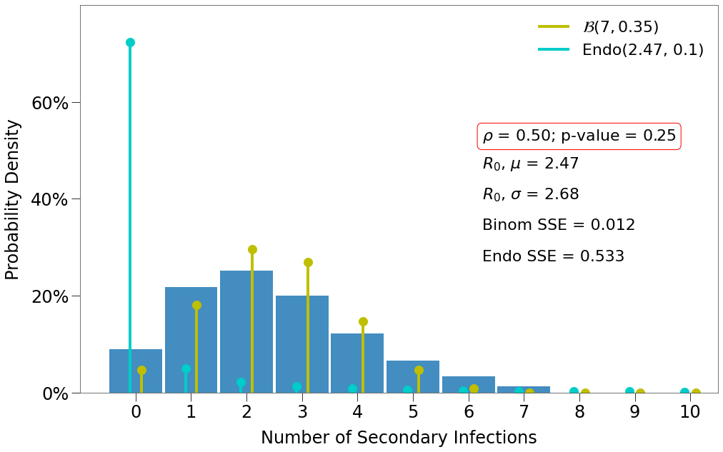
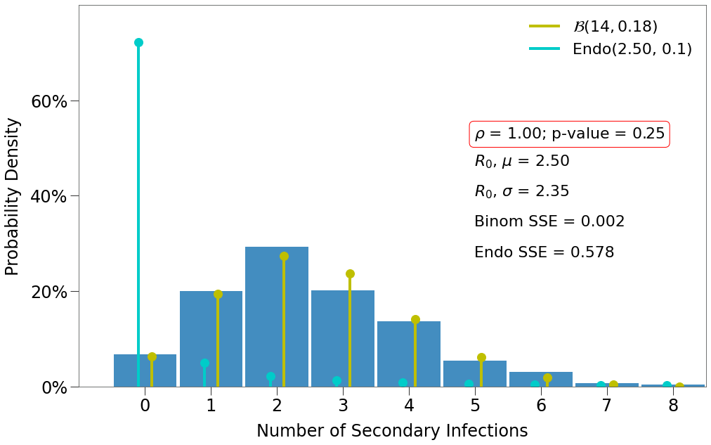
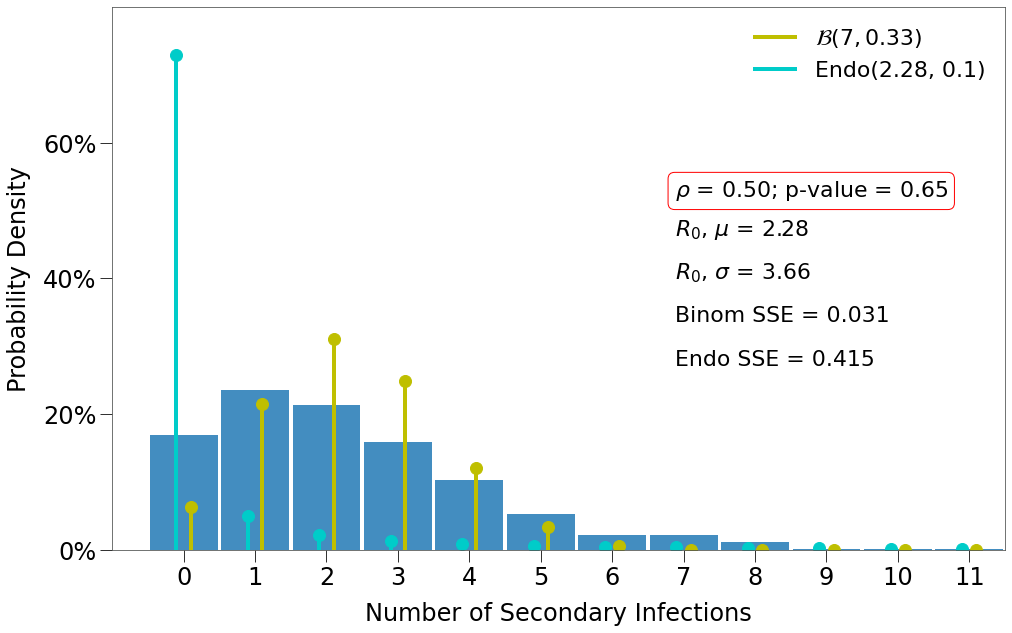
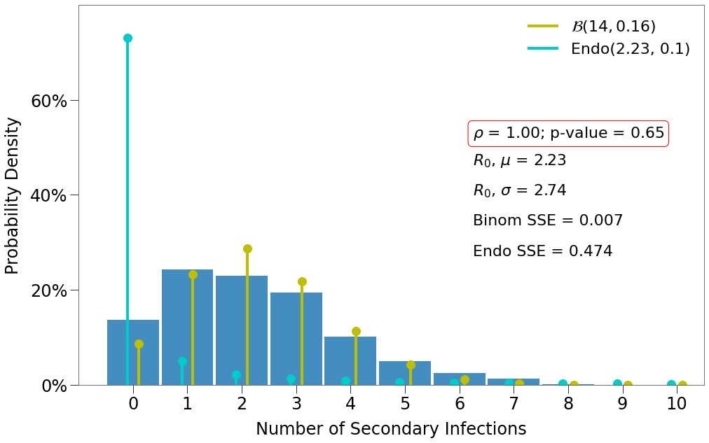
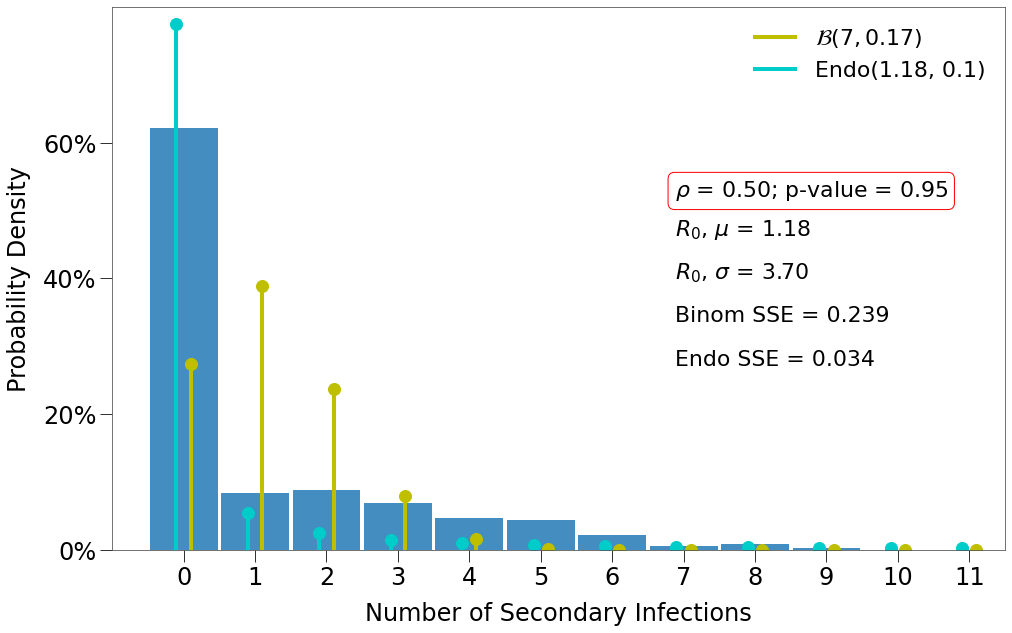
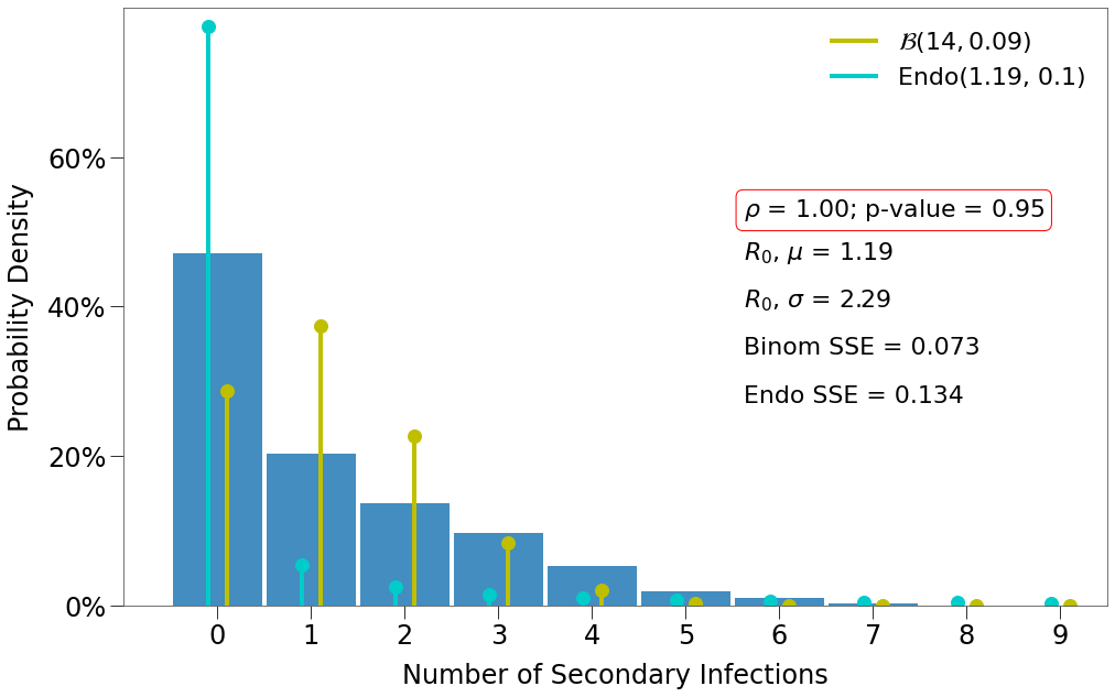
Here we have a few findings:

There is one decent fit for the Endo model, which comes at the lowest density and the highest p-value.
The closest fit to the Binomial distribution comes at density=1 and the lowest p-value.

Complex Environments¶

We can use our findings to structure more complex environments that more appropriately mock real world interactions.

Here, we will incorporate a dynamic transmission curve with $R_0$ dispersion that fits the Endo model.

$\underline{\text{Hutch}}$

As noted previously, with respect to sars-cov-2, the Hutch model uses a Gamma distribution to govern real world interactions as per below:

\[\begin{split}\begin{equation} c_t\;\approx\;\Gamma(\alpha, \theta)\;\approx\;\Gamma(\frac{\overline{k}}{\theta}, \theta) \\\alpha \textit{ is the shape parameter, } \\\mu = \overline{k}, \textit{or the average daily contact rate } \\\theta\textit{ is the dispersion parameter} \end{equation}\end{split}\]

The scaling parameters are related to mean and variance as follows:

\[\begin{split}\begin{equation} \\\overline{k} = \alpha\theta \\\sigma^2 = \alpha\theta^2 \end{equation}\end{split}\]

The Hutch model combines this approach to contact distributions with a model for dynamic viral load to estimate contact level parameters for viral transmission.

They detail two sets of parameters for two $R_0$ outcomes.

$\underline{R_0 = 1.8}$

mean $R_0$ of 1.8
4 mean contacts per day, $\overline{k}$
40 dispersion, $\theta$
$\lambda$ of 10**7 (a parameter influencing the relative infectiousness of an infected subjected)

$\underline{R_0 = 2.8}$

mean $R_0$ of 2.8
20 mean contacts per day, $\overline{k}$
30 dispersion, $\theta$
$\lambda$ of 10**7.5

The parameter best fit for both outcomes was determined on a number of external inputs including adherence to the findings of the Endo model that >70%+ primary infections caused no secondary infections.

Limitation

Currently, RKnot cannot replicate $R_0$ of 2.8 according to the above parameters as it cannot generate $\overline{k}=20$ according to the required Gamma distribution. This will be more viable when multiple ticks per day are available.

$\underline{\text{Process}}$

Our goal is to replicate both the Hutch model gamma distribution (both $\overline{k}$ and $\theta$) and the Endo model $R_0$ distribution.

RKnot currently has 4 tools for increasing contact rate:

changing density
changing movement patterns
events
vboxes

We have seen that increasing density does increase $\overline{k}$, but that both contacts and $R_0$ are normally/binomially distributed. So increasing density is not appropriate.

We have also seen that changing movement patterns only has an impact where density < 1 and can only increase it up to the density. So, if our density must be <= 1, our movement pattern can only ever increase density to <= 1.

So we are left with events and vboxes.

Thus, our process for building complex environments is as follows:

Process

Identify required contact distribution based on Hutch parameters.
Identify contact distribution to result from events.
Determine the number of events required for each capacity to replicate the curve from 2) above.
Determine the density of the remaining dots not in the vbox and find mover function that helps replicate the required contact distribution at the lower contact levels.
Set the vbox location size based on maximum number of events per day.

Hutch Model: $R_0$ of 1.8¶

We will demonstrate the building of a complex environment using $R_0$ 1.8 Hutch model.

Our environment will have with following initial conditions:

Population of 10,000
Initial infected of 1
Density of 1
Length of 30 days
0.98 p-value for mover

Our model targets: + $R_0 = 1.8$ + $\overline{k} = 4$ + $\theta = 40$

$\underline{\text{Exploring the Contact Distribution}}$

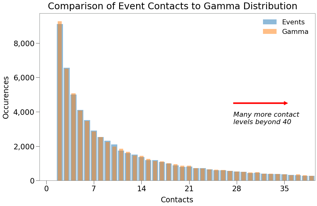
We can visualize the expected contact rate distribution by generating a random set of contacts on the gamma distribution.

We know that there should be $n_{dots}$ * $n_{days}$ number of records of contacts (300,000) and so can show the number of occurences of each amount of contacts from a gamma sample:

The initial parameters are as follows:

[39]:

n = 10000
days = 30
size = n*days
density = 1
gloc = 2
sim_tmr = tmr

mu = 4
theta = 40
tgt_R0 = 1.8

From these, we can generate a sample gamma distribution as follows:

[40]:

alpha = mu / theta
k_gam = np.random.gamma(alpha, size=size, scale=theta)

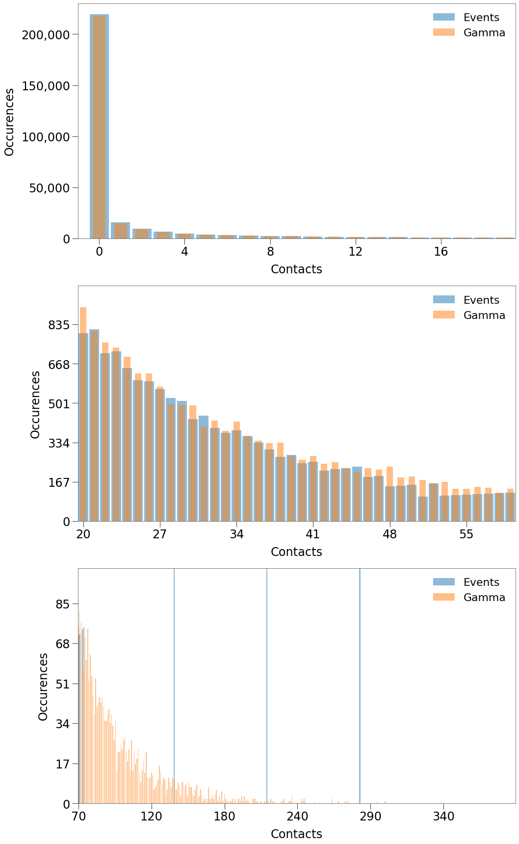
k_gam can be passed to a histogram and results in the folllowing:

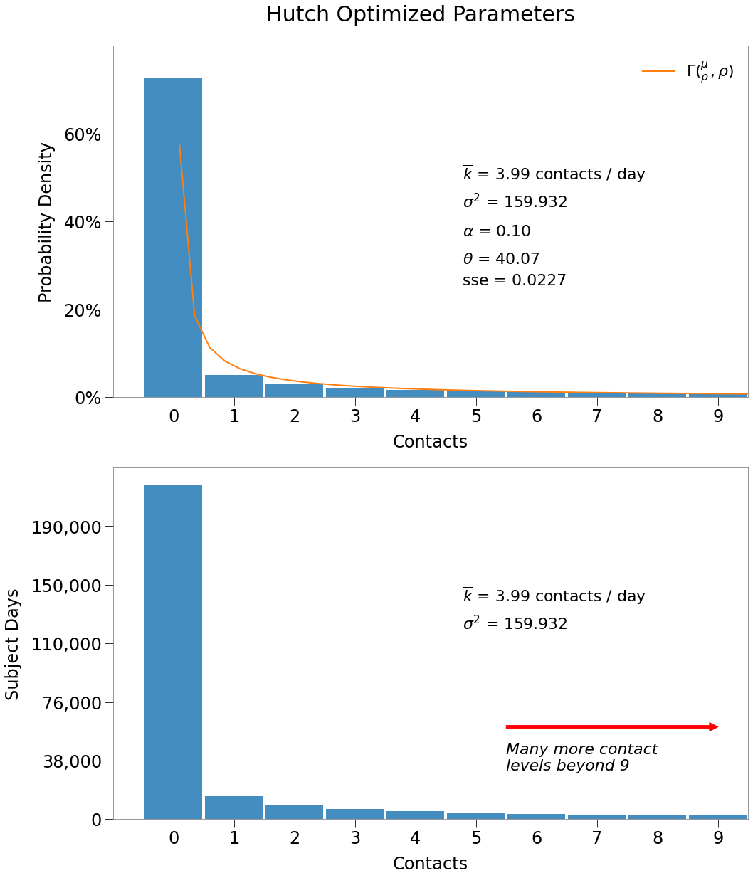
By far, most dot-days must have 0 contacts. Above we zoomed in on the first 10 contact levels to give a sense for the most pertinent values.

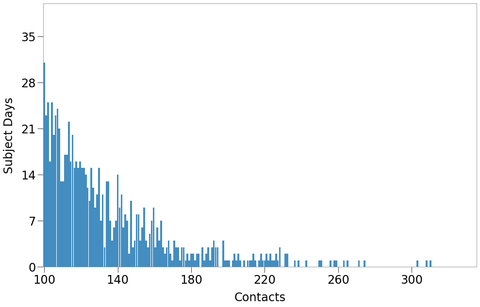
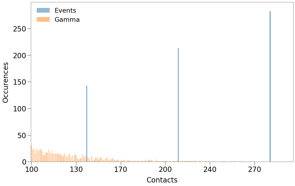
Below we show the distribution tail. Remember that while the number of occurences is relatively low, given the contact level is so high they still produce a large number of contacts.

For instance:

2,000 dot-days of 2 contacts produces 4,000 contacts
40 dot-days of 100 contacts produces 40,000 contacts

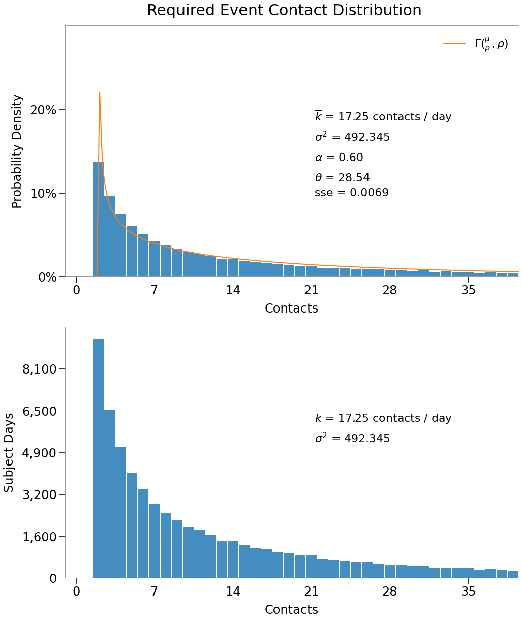
From the distribution above, we can focus on the contacts that must be event-driven. For our sim, we have chosen contacts of 2 or more (equal to event apacity of 3) to result from events.

Thus, events must replicate the distribution below, which is still a gamma distribution, slightly modified from the original.

$\underline{\text{Creating Events}}$

The number of contacts for a single dot at an event is simply the capacity minus 1, since a dot cannot contact itself.

\[\begin{split}\begin{equation} k_e = \text{cap}_e - 1 \\\textit{where: } k_e \textit{ = contact level for event e} \\\textit{cap}_e \textit{ = capacity for event e} \end{equation}\end{split}\]

Multiplying again for every dot at the event gives us the total contacts for all dots:

\[\begin{split}\begin{equation} c_e\;=\;(cap_e - 1)*cap_e \\\textit{where: } c_e \textit{ = total contacts for event e} \end{equation}\end{split}\]

Remember that our target $\overline{k}$ is the average contact rate per dot, so the number of events should be structured on a per dot basis. The number of events required for a particular contact level, $k$, then, is:

\[\begin{split}\begin{equation} n_{e,j} = \frac{k_{tgt,i}}{cap_{e,j}} \\\textit{i = contact level} \\\textit{j = i + 1 = event capacity} \end{equation}\end{split}\]

[44]:

c_eve = c_eve.astype(np.int32)
caps = np.arange(c_eve.shape[0]) + 1

n_events = c_eve[gloc:] / caps[gloc:]

RKnot’s ability to replicate the Gamma distribution fails on the long tail of the distribution when the number of occurences of a specified contact level is fewer than the contacts that would be generated by a single event.

For instance, the Hutch gamma distribution results in ~40 dot-days with 100 contacts. RKnot can only generate 100 contacts through a 100 contact event and a 100 contact event generates $(100-1)*100 = 9,900$ contacts, far more than required.

Our current hack-fix is to regroup and redistribute all contact occurences above that threshold into events. This results in a tail that is less evenly distributed.

A better solution would be to increase the number of ticks per day, which would allow for many more independent streams of contact distributions among dots. This feature will be available in future versions.

[45]:

i_events = np.argwhere(n_events < 1 ).ravel()

i_large = i_events[0]

k_to_replicate = n_events[i_large:]*caps[gloc + i_large:]*caps[gloc + i_large:]

total = k_to_replicate.sum()
skip = 70
add_caps = []
for cap in range(i_large + skip + 1, i_large + k_to_replicate.shape[0] + 1, skip):
    total = total - ((cap - 1)*cap)
    if total < 0:
        break
    else:
        add_caps.append(cap)
        n_events[cap - 1] = 1

n_events = np.where(n_events >= 1, n_events, 0).astype(np.int32)

With the number of events for each capacity determined, we can assign event objects.

To do so, we:

utilize the “baseus” groups used in the SIR analysis.
assign a p-value of .98 to the mover function of group.
- determined through a trial and error process that best fit the Hutch distribution.
randomly assign each event a start tick between 1 and 30, which is the length of the simulation.
assign each event to vbox=0
as all events will occur inside a vbox, a Travel event must be used to transport them to the event location.

from rknot.sims import baseus
from rknot.events import Travel

groups = baseus.groups
groups[2]['n_inf'] = 0
for group in groups:
    group['mover'] = .98

params = {'days': days, 'tmr_curve': sim_tmr, 'density': density, 'sterile': True}

event_groups = []
for i in np.arange(n_events.shape[0]):
    if n_events[i] >= 1:
        event_group = {'name': f'{i+gloc+1}n', 'n': n_events[i], 'groups': [0,1,2,3], 'capacity': i+gloc+1}
        event_groups.append(event_group)

events = []
for i, e in enumerate(event_groups):
    for j in range(e['n']):
        start_tick = np.random.randint(1, 31, 1, dtype=np.int32)
        events.append(
            Travel(name='{}_{}'.format(e['name'], j), start_tick=start_tick[0], groups=e['groups'], capacity=e['capacity'], vbox=0)
        )

In the chart below, we can see the distribution of the capacity of the events generated by this process over the life of the simulation.

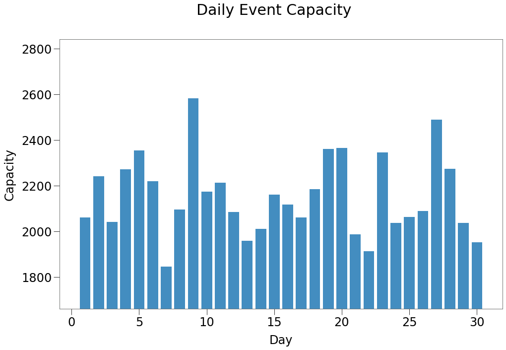
So, for the length of the simulation between 18 to 26% of the population will be attending events each day of the simulation.

Below, we can see that for the lower contact levels, this approach generates a near perfect replica of the required Gamma distribution.

When we focus on contact levels of 100+, however, you can see that we only generate contacts at 3 levels.

$\underline{\text{Forming the Remaining Environment}}$

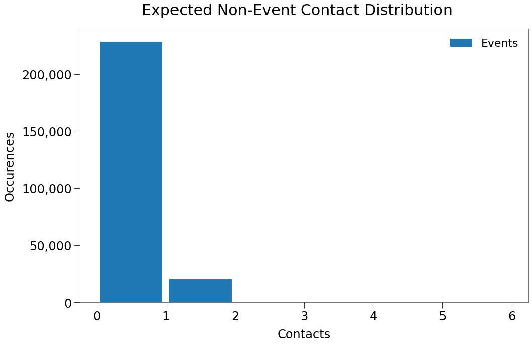
With contact levels 2+ settled, we must set the non-event environment such that it generates mainly 0 contacts.

First, we find the average density of the grid (excluding the vbox) during the sim. Only dots not attending events will be in the main grid, so density is as follows:

[51]:

n_dots_at_events = np.array(list(c.values())).mean()
n_dots_not_events = n - n_dots_at_events

d = n_dots_not_events / n # given density of 1

print (np.around(d, 2))

0.78

The density of the grid excluding dots on events will be 0.78.So we can find the expected $\overline{k}$ of that space using the polyfit equation we found above to find the corresponding variance and providing the p-value for group movement. And then apply $\overline{k}$ to a normal distribution to find the expected contacts for the non-event space.

[54]:

f = np.poly1d(d*z)
mu_space = f(.98)
var_space = mu_space
x = np.linspace(0, 5, 6)
c_non = st.norm.pdf(x, mu_space, np.sqrt(var_space))
c_non = d*n*30*c_non

[57]:

text = 'And so the expect 0 contacts occurences are right in line with the target: '
text += f'\n\n {c_non[0]:,.0f} vs. {c_gam[0]:,.0f}'
text += '\n\nThere is greater delta in the 1 contact occurences but still fairly close: '
text += f'\n\n {c_non[1]:,.0f} vs. {c_gam[1]:,.0f}'

md(text)

And so the expect 0 contacts occurences are right in line with the target:

228,464 vs. 217,740

There is greater delta in the 1 contact occurences but still fairly close:

20,230 vs. 15,090

Thus, we expect the non-event space will result in 200,000+ dot days with no contacts, right in line with Hutch gamma.

The final step in preparing the simulation environment is determing the size of the VBox. The chart below shows the number of events occuring on each tick in the Sim.

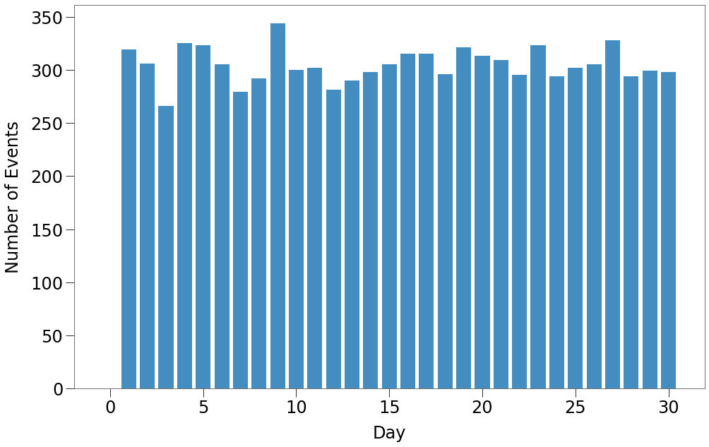
Above we can see that there are typically ~300 events occuring on a given tick.

The vbox must allow for each event to have its own location, so the vbox should have enough locations to support the maximum number of events occuring on the same tick, which is:

[59]:

start_ticks = np.array([e.start_tick for e in events])
n_events_by_tick = np.bincount(start_ticks)
n_events_by_tick.max()

[59]:

The vbox must have 344 locations.

$\underline{\text{Run the Sim}}$

We will run a single Sim to use for all_contacts comparison:

vbox = n_events_by_tick.max()
sim = Sim(groups=groups, events=events, vboxes=vbox, **params)
sim.run(dotlog=True)

all_contacts = find_all_contacts(sim.dotlog, MLNB)
eR0_all = np.sum(all_contacts[:,:sim_tmr.shape[0]]*sim_tmr, axis=1).mean()

We can see from the outputs that the sim produces fairly similar outcomes to those desired.

$\underline{\text{Results}}$

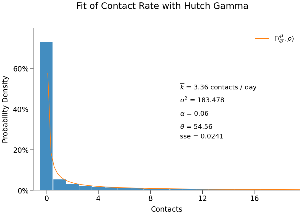
The sim reproduced $R_0$ as desired, however, contact rate is slightly below target and theta slightly over. This is likely the result of the long-tail issues described earlier.

$R_0$	$\overline{{k}}$	$\theta$
1.82	3.36	54.56

And the contact distribution visually fits the desired Gamma almost perfectly (except for contact levels > 100 as previously noted).

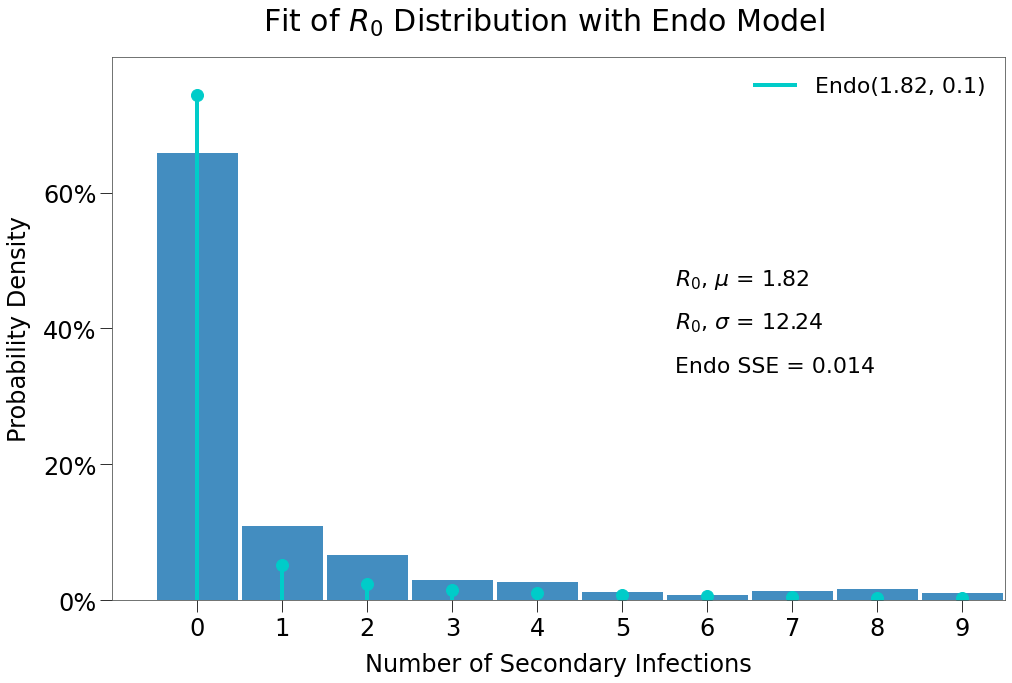
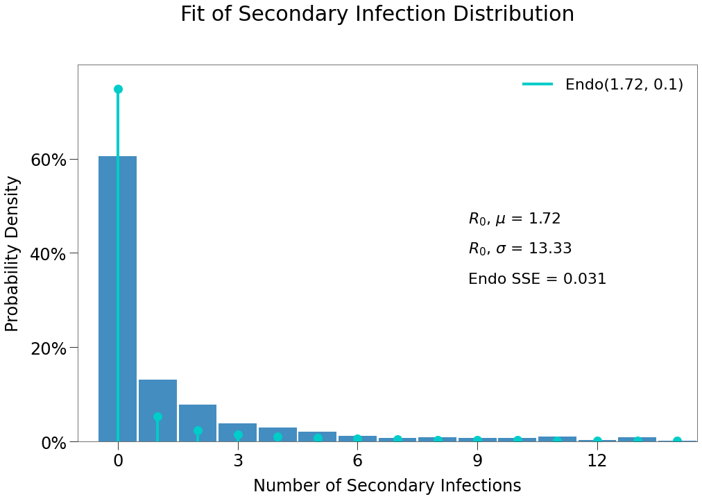
And that the expected $R_0$ distribtion is a much stronger fit for the Endo model (although still underweight slightly to 0 infection outcomes).

$\underline{\text{Run a Larger Dataset}}$

The all_contacts method is good way to get a quick read on the viability of an environment, however, it is still only a rough estimate. Truly reliable statistics can only come from running the simulation many times.

We will loop through 1,000 sims:

n = 1000
contacts, nsecs, results, exceptions = looper(groups, n, params['density'], params['days'], tmr=sim_tmr, events=events, vboxes=vbox)

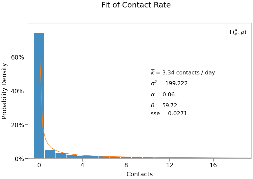
$\underline{\text{Results}}$

[68]:

eR0 = np.mean(contacts.reshape(-1,sim_tmr.shape[0])*sim_tmr, axis=0).sum()
R0 = nsecs.sum(axis=1).mean()

E($R_0$)	$R_0$	$\overline{{k}}$	$\theta$
1.78	1.72	3.34	59.72

The above iterations set sterile=True, in order to isolate the contacts and secondary infections of just the initial infected.

We can learn more about the outcomes in the simulation by again using looper and setting sterile=False, days=365. We will complete just 250 iterations, because each sim will run longer.

n = 250
days = 365
contacts, nsecs, results, exceptions = looper(groups, n, density, days, tmr=sim_tmr, events=events, vboxes=vbox, sterile=False)

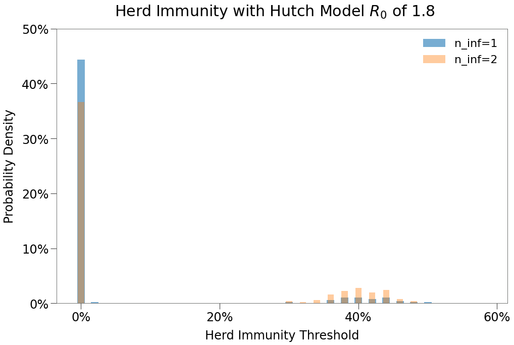
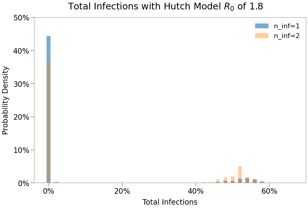
	1 Infection	2 Infections	1 Infection $R_0$ > 0	2 Infections $R_0$ > 0
Peak	3.8%	8.9%	34.5%	33.1%
HIT	4.6%	11.1%	42.3%	41.1%
Total	5.9%	14.0%	53.8%	52.3%
Days to Peak	11	24	28	38